42. Pareto Distributions and Aggregate Production Functions#
42.1. Overview#
Macroeconomic models often describe an industry, or a whole economy, with a smooth production function in which inputs substitute for one another.
Yet many individual machines and plants work with nearly fixed proportions.
A spinning frame needs a given amount of power and labor per pound of yarn, and adding workers to an idle frame produces no more yarn.
Houthakker [1955] showed how the two descriptions fit together.
He studied an industry made of many small production cells, each with fixed input proportions and a capacity set by its fixed inputs, and with proportions that differ from cell to cell.
When input prices change, some cells start producing and others stop, so the industry’s mix of inputs changes even though no single cell’s mix does.
Substitution at the level of the industry comes from changes in which cells operate.
Houthakker’s main result is that if the cells’ input coefficients follow a Pareto distribution, then the industry’s aggregate production function is Cobb–Douglas.
The exponents of that Cobb–Douglas function are not properties of any cell’s technology: they are parameters of the distribution of cells.
So an aggregate production function can look smooth and stable although no cell substitutes, and it moves whenever entry, exit or investment changes the distribution.
Levhari [1968] turned the question around: given an aggregate production function, which distribution of cells generates it?
He answered it for a CES production function.
In this lecture we
prove Houthakker’s efficiency theorem: if every cell maximizes profit at the same prices, the industry’s total inputs and output are efficient;
derive Houthakker’s Cobb–Douglas production function and identify the property of the Pareto distribution that delivers it;
compute the aggregate production function of a finite set of cells as a linear program, in the spirit of the activity analysis of Koopmans [1951];
use the program’s dual to write the aggregate production function of any distribution of cells as a minimization over prices, which can be computed even where Houthakker saw no general way to eliminate the prices;
reproduce Levhari’s inversion, give a general formula for it, and correct his description of the shape of the distribution that generates a CES production function.
The lecture uses linear programming and duality, as in Linear Programming, Optimal Transport and Von Neumann Growth Model (and a Generalization), Pareto tails, as in Heavy-Tailed Distributions, and Lorenz curves, as in Wealth Distribution Dynamics.
We use the following imports.
import numpy as np
import matplotlib.pyplot as plt
from scipy import integrate
from scipy.optimize import linprog, brentq, minimize
from scipy.special import beta as beta_function, gamma as gamma_function
42.2. Production cells#
Houthakker considers an industry made of many production cells.
A cell can be a firm, a plant, a single machine, or a worker.
Each cell produces an output \(x_0\) with two variable inputs \(x_1\) and \(x_2\) and with some fixed inputs.
The fixed inputs cannot be changed during the period studied.
They define the cell and limit what it can produce.
(Houthakker allows several outputs and many variable inputs, but he soon specializes to one output and two variable inputs, and so do we.)
Summing over cells gives the industry’s total output \(X_0\) and total variable inputs \(X_1\) and \(X_2\).
Houthakker does not sum the fixed inputs, which may not even be measurable.
A total \((X_0, X_1, X_2)\) is attainable if the cells, with the fixed inputs they have, can jointly produce \(X_0\) from \(X_1\) and \(X_2\).
Following Koopmans, an attainable total is efficient if no other attainable total has at least as much output, at most as much of each input, and is strictly better in at least one of these three respects.
Theorem 42.1 (Efficiency (Houthakker’s theorem))
Let the price of output be \(p_0 > 0\) and the prices of the variable inputs be \(p_1 > 0\) and \(p_2 > 0\).
If each cell chooses, among its production possibilities, one that maximizes its profit \(p_0 x_0 - p_1 x_1 - p_2 x_2\), then the industry’s total \((X_0, X_1, X_2)\) is efficient.
Among all attainable totals, it also maximizes the industry’s total profit.
Proof. Total profit \(p_0 X_0 - p_1 X_1 - p_2 X_2\) is the sum of the cells’ profits.
Each cell’s profit is as large as it can be, so no attainable total earns more.
Suppose that another attainable total \((X_0', X_1', X_2')\) had \(X_0' \geq X_0\), \(X_1' \leq X_1\), \(X_2' \leq X_2\), with at least one strict inequality.
Because all prices are positive, it would earn strictly more profit than \((X_0, X_1, X_2)\), which is impossible.
The proof uses nothing about the cells except that each maximizes profit.
It is a version of the first welfare theorem for producers.
With one output, every efficient total lies on the graph of an aggregate production function
the largest output the industry can attain from total inputs \(X_1\) and \(X_2\), given the fixed inputs of its cells.
Where \(F\) increases strictly in both inputs, as it does in Houthakker’s case below, the efficient totals are exactly this graph.
Theorem 42.1 says that price-taking cells put the industry on this function.
42.3. Fixed coefficients#
From now on, each cell has fixed coefficients.
A cell needs \(a_1\) units of \(x_1\) and \(a_2\) units of \(x_2\) to produce one unit of output, and it can produce any amount between zero and a capacity set by its fixed inputs.
The coefficients \(a = (a_1, a_2)\) differ across cells.
A proportional change in all prices affects no cell’s choice, so we set \(p_0 = 1\) and write \(p = (p_1, p_2)\).
A cell with coefficients \(a\) earns \(1 - a_1 p_1 - a_2 p_2\) on each unit it produces.
If this is positive, the cell produces to capacity; if it is negative, the cell produces nothing.
Houthakker assumes that cells are small and numerous, so that the cells exactly on the margin, which earn zero, can be neglected.
In the \((a_1, a_2)\) plane, the cells that produce are those in the price triangle below the line \(a_1 p_1 + a_2 p_2 = 1\), which meets the axes at \(1/p_1\) and \(1/p_2\).
Houthakker summarizes the cells by their input–output distribution \(\varphi\): the cells whose coefficients lie in a small rectangle \([a_1, a_1 + da_1] \times [a_2, a_2 + da_2]\) have total capacity \(\varphi(a_1, a_2) \, da_1 \, da_2\).
Integrating over the price triangle gives the industry’s output and inputs at prices \(p\):
These are three equations in two prices.
Eliminating the prices leaves one relation among \(X_0\), \(X_1\) and \(X_2\).
By Theorem 42.1, the totals that profit-maximizing cells produce are efficient, so that relation is the aggregate production function.
The industry profit function
adds up the cells’ profits.
A cell’s fixed inputs are what limit its output, so its profit is the return to those inputs, which Marshall called a quasi-rent.
Differentiating under the integral gives Hotelling’s lemma, \(\partial \Pi / \partial p_i = -X_i(p)\): the derivative of the industry’s profit with respect to an input price is minus the industry’s use of that input.
\(\Pi\) is convex in \(p\) because it integrates convex functions of \(p\).
We return to \(\Pi\) below.
42.4. A Pareto distribution#
Houthakker assumes that the input–output distribution is
with constants \(A > 0\), \(\alpha_1 > 0\) and \(\alpha_2 > 0\).
(Houthakker requires \(\alpha_i \geq 1\), but the derivation below needs only \(\alpha_i > 0\).)
The name comes from the distribution of productivities.
With one variable input and coefficient \(a\), a cell gets \(y = 1/a\) units of output from each unit of input.
Under the one-input version of (42.3), \(\varphi(a) = A a^{\alpha - 1}\), the cells whose productivity exceeds \(y\) have total capacity
which is Pareto’s law for the number of incomes that exceed \(y\).
Total capacity, \(\iint \varphi(a) \, da\), is infinite: there is an unlimited supply of ever less productive cells.
At any positive prices only the cells inside the price triangle matter, and their total capacity is finite.
42.4.1. Deriving the Cobb–Douglas form#
To compute \(X_0\), integrate over \(a_2\) first and then substitute \(\tau = a_1 p_1\):
where \(B\) is the beta function.
The same steps give \(X_1\) and \(X_2\).
Let \(D = A \, B(\alpha_1 + 1, \alpha_2 + 1)\).
The identity \(B(x, y) = \frac{x + y}{x} B(x + 1, y)\) gives \(B(\alpha_1, \alpha_2 + 1) = \frac{1 + \alpha_1 + \alpha_2}{\alpha_1} B(\alpha_1 + 1, \alpha_2 + 1)\), and Houthakker writes the results as
(In the paper, the formula for \(X_2\) is misprinted with the label \(X_1\).)
Dividing shows that each input’s share of the value of output is constant:
Substituting \(p_i = \gamma_i X_0 / X_i\) into the formula for \(X_0\) gives an equation with \(X_0\) on both sides; solving it leaves
This is Houthakker’s Cobb–Douglas production function.
Three features of it deserve comment.
First, the marginal product of input \(i\) is \(\gamma_i X_0 / X_i = p_i\), as Theorem 42.1 requires.
Second, the exponents add up to \((\alpha_1 + \alpha_2)/(1 + \alpha_1 + \alpha_2) < 1\).
Returns to the variable inputs diminish because the fixed inputs are held fixed, and the fixed inputs receive the remaining share \(1/(1 + \alpha_1 + \alpha_2)\) of output as quasi-rents \(\Pi\).
Third, adding a fictitious input \(X_3\) with exponent \(1/(1 + \alpha_1 + \alpha_2)\) would make the function homogeneous of degree one.
Houthakker warns that this would mislead: what matters is how the fixed inputs are distributed across cells, not their total.
42.4.2. Why a Pareto distribution gives a Cobb–Douglas function#
The reason is a scaling property.
Lowering \(p_1\) to \(p_1 / \lambda\) stretches the price triangle by the factor \(\lambda\) in the \(a_1\) direction.
Under (42.3), \(\varphi(\lambda a_1, a_2) = \lambda^{\alpha_1 - 1} \varphi(a_1, a_2)\), so the cells in the stretched triangle look like the cells in the old triangle, rescaled.
Changing variables to \(a_1 = \lambda \tilde a_1\) in (42.1) shows that \(X_0\) and \(X_2\) are multiplied by \(\lambda^{\alpha_1}\) and \(X_1\) by \(\lambda^{\alpha_1 + 1}\).
Hence \(p_1 X_1 / X_0\) does not change when \(p_1\) changes, and the same argument applies to \(p_2\).
Each input’s share is therefore constant.
Since each share equals the elasticity \(\partial \log F / \partial \log X_i\), a production function with constant shares is Cobb–Douglas.
The property that does the work is that \(\varphi\) scales as a power separately in \(a_1\) and in \(a_2\).
Exercise 42.1 shows that scaling in \((a_1, a_2)\) jointly is not enough.
42.4.3. Checking the formulas#
The function below evaluates (42.4), and the next one evaluates (42.6).
def pareto_totals(p, A, α):
    """Industry output and inputs (X0, X1, X2) at input prices p."""
    (p1, p2), (α1, α2) = p, α
    D = A * beta_function(α1 + 1, α2 + 1)
    X0 = (1 + α1 + α2) * D / (α1 * α2 * p1**α1 * p2**α2)
    X1 = D / (α2 * p1**(α1 + 1) * p2**α2)
    X2 = D / (α1 * p1**α1 * p2**(α2 + 1))
    return X0, X1, X2


def cobb_douglas(X1, X2, A, α):
    """Houthakker's aggregate production function."""
    α1, α2 = α
    n = 1 + α1 + α2
    D = A * beta_function(α1 + 1, α2 + 1)
    C = n * (D / (α1**(α1 + 1) * α2**(α2 + 1)))**(1 / n)
    return C * X1**(α1 / n) * X2**(α2 / n)
As an independent check, we compute the integrals (42.1) numerically.
def totals_by_quadrature(p, φ):
    """Integrate φ, a1 φ and a2 φ over the price triangle."""
    p1, p2 = p
    limits = (0, 1 / p1, 0, lambda a1: (1 - a1 * p1) / p2)
    X0 = integrate.dblquad(lambda a2, a1: φ(a1, a2), *limits)[0]
    X1 = integrate.dblquad(lambda a2, a1: a1 * φ(a1, a2), *limits)[0]
    X2 = integrate.dblquad(lambda a2, a1: a2 * φ(a1, a2), *limits)[0]
    return X0, X1, X2
We use \(A = 1\), \(\alpha_1 = 2\) and \(\alpha_2 = 1.5\) throughout, so that \(\gamma_1 = 4/9\), \(\gamma_2 = 1/3\) and the fixed inputs’ share is \(2/9\).
A, α = 1.0, (2.0, 1.5)
φ = lambda a1, a2: A * a1**(α[0] - 1) * a2**(α[1] - 1)

print(f"{'p':12} {'X0 (quad)':>10} {'X0 (formula)':>12} {'F(X1, X2)':>11} "
      f"{'p1 X1/X0':>9} {'p2 X2/X0':>9}")
for p in [(1.0, 1.0), (0.7, 1.6), (2.0, 0.8)]:
    X0_q, _, _ = totals_by_quadrature(p, φ)
    X0, X1, X2 = pareto_totals(p, A, α)
    print(f"{str(p):12} {X0_q:10.6f} {X0:12.6f} "
          f"{cobb_douglas(X1, X2, A, α):11.6f} "
          f"{p[0] * X1 / X0:9.4f} {p[1] * X2 / X0:9.4f}")
p             X0 (quad) X0 (formula)   F(X1, X2)  p1 X1/X0  p2 X2/X0
(1.0, 1.0)     0.076190     0.076190    0.076190    0.4444    0.3333
(0.7, 1.6)     0.076829     0.076829    0.076829    0.4444    0.3333
(2.0, 0.8)     0.026620     0.026620    0.026620    0.4444    0.3333
The formulas match the numerical integrals, the Cobb–Douglas function (42.6) reproduces output from the inputs, and the shares are \(4/9\) and \(1/3\) at every price vector.
42.5. Activity analysis with finitely many cells#
Houthakker’s title places his note in activity analysis, the study of production as a choice among linear activities that Koopmans [1951] and his colleagues developed.
With finitely many cells, his aggregation becomes a linear program.
42.5.1. The aggregate production function as a linear program#
Let cell \(j = 1, \ldots, N\) have capacity \(c_j\) and coefficients \(a_j = (a_{1j}, a_{2j})\), and let it run at intensity \(z_j \in [0, 1]\), the fraction of its capacity that it uses.
The largest output attainable from inputs \(X = (X_1, X_2)\) is
Attach multipliers \(p_i \geq 0\) to the two input constraints and \(\mu_j \geq 0\) to the capacity constraints \(z_j \leq 1\).
The dual program is
For given \(p\), the smallest feasible \(\mu_j\) is \(c_j \max\{0, 1 - a_j \cdot p\}\), the quasi-rent of cell \(j\) at prices \(p\).
Substituting it, and using the duality theorem of linear programming, which says that the two programs have the same optimal value (see Optimal Transport), gives
This formula teaches four things.
First, weak duality gives Theorem 42.1.
At any prices \(p \geq 0\), each cell’s output is at most its input cost plus its quasi-rent, so any feasible intensities produce at most \(p \cdot X + \Pi_N(p)\).
Cells that maximize profit at \(p\) attain this bound with their own inputs \(X\), so no attainable total does better.
Complementary slackness, as in Optimal Transport, gives the converse: at the optimal dual prices every cell with \(a_j \cdot p < 1\) runs at capacity and every cell with \(a_j \cdot p > 1\) is idle, so every efficient total is one that profit-maximizing cells can produce at some prices.
Second, the same holds with a continuum of cells.
The same argument, with integrals in place of sums, gives \(F(X) = \min_{p \geq 0} \{ p \cdot X + \Pi(p) \}\), with \(\Pi\) from (42.2), for every input vector \(X\) that some prices generate.
Under Houthakker’s distribution, that is every \(X > 0\).
Going the other way, \(\Pi(p) = \max_X \{ F(X) - p \cdot X \}\), so the aggregate production function and the industry profit function are dual to each other, and each can be recovered from the other.
Third, the formula gives a numerical method, not a closed form.
Houthakker wrote that “there appears to be no generally applicable method of eliminating \(p_1\) and \(p_2\)” from his versions of (42.1) “and thus deriving \(F\) directly from \(\varphi\).”
The minimization does not eliminate the prices in closed form: by Hotelling’s lemma, its first-order conditions are exactly the equations \(X_i(p) = X_i\).
What it adds is a convex problem in two variables, which is easy to solve numerically for any \(\varphi\), and which still makes sense with finitely many cells, where the equations \(X_i(p) = X_i\) usually have no exact solution.
Fourth, \(F_N\) is concave and piecewise linear, so its isoquants are piecewise linear too.
As \(N\) grows with cells drawn from \(\varphi\), they approach the smooth isoquants of \(F\).
To illustrate the third point, we compute \(F\) for Houthakker’s distribution by minimizing \(p \cdot X + \Pi(p)\) over prices, evaluating \(\Pi\) by numerical integration rather than from the closed forms.
We search over \(\log p\) to keep prices positive.
def profit_by_quadrature(p, φ):
    """Industry profit Π(p) from (ha_profit), by numerical integration."""
    p1, p2 = p
    return integrate.dblquad(
        lambda a2, a1: (1 - a1 * p1 - a2 * p2) * φ(a1, a2),
        0, 1 / p1, 0, lambda a1: (1 - a1 * p1) / p2)[0]


def F_by_duality(X, φ):
    """Minimize p·X + Π(p) over p > 0; return the value and the prices."""
    def objective(log_p):
        p = np.exp(log_p)
        return p @ X + profit_by_quadrature(p, φ)
    res = minimize(objective, np.zeros(2), method="Nelder-Mead",
                   options={"xatol": 1e-8, "fatol": 1e-12})
    return res.fun, np.exp(res.x)


print(f"{'X':14} {'min p·X + Π(p)':>15} {'Cobb–Douglas':>13}   prices")
for X in ([0.03, 0.025], [0.05, 0.02]):
    value, p = F_by_duality(np.array(X), φ)
    print(f"{str(X):14} {value:15.8f} {cobb_douglas(*X, A, α):13.8f}   "
          f"({p[0]:.4f}, {p[1]:.4f})")
X               min p·X + Π(p)  Cobb–Douglas   prices
[0.03, 0.025]       0.07181985    0.07181985   (1.0640, 0.9576)
[0.05, 0.02]        0.08366438    0.08366438   (0.7437, 1.3944)
The minimization reproduces the Cobb–Douglas function, and the minimizing prices are the marginal products \(\gamma_i X_0 / X_i\).
42.5.2. Drawing cells from Houthakker’s distribution#
Total capacity under (42.3) is infinite, so we cannot draw cells from all of it.
Instead we keep the cells in a large triangle \(a_1/\bar a_1 + a_2/\bar a_2 \leq 1\).
This contains the price triangle whenever \(p_1 \geq 1/\bar a_1\) and \(p_2 \geq 1/\bar a_2\), and at those prices the truncation changes nothing.
Inside the large triangle, the scaled coefficients \((a_1/\bar a_1, a_2/\bar a_2)\) have density proportional to \(b_1^{\alpha_1 - 1} b_2^{\alpha_2 - 1}\) on the set \(b_1 + b_2 \leq 1\).
That is the distribution of the first two coordinates of a Dirichlet random vector with parameters \((\alpha_1, \alpha_2, 1)\).
The large triangle is the price triangle at \(p = (1/\bar a_1, 1/\bar a_2)\), so its total capacity is \(X_0(1/\bar a_1, 1/\bar a_2) = A \, \bar a_1^{\alpha_1} \bar a_2^{\alpha_2} \, \Gamma(\alpha_1) \Gamma(\alpha_2) / \Gamma(1 + \alpha_1 + \alpha_2)\), where \(\Gamma\) is the gamma function; we split it equally among \(N\) cells.
ā = np.array([2.0, 2.0])


def draw_cells(N, A, α, ā, rng):
    """N cells from φ restricted to the triangle a1/ā1 + a2/ā2 <= 1."""
    b = rng.dirichlet([α[0], α[1], 1.0], size=N)[:, :2]
    total = (A * ā[0]**α[0] * ā[1]**α[1] * gamma_function(α[0])
             * gamma_function(α[1]) / gamma_function(1 + α[0] + α[1]))
    return ā * b, np.full(N, total / N)


def F_lp(X, a, c):
    """Solve the linear program (ha_lp); return output and dual prices."""
    res = linprog(-c, A_ub=(a * c[:, None]).T, b_ub=X,
                  bounds=(0, 1), method="highs")
    if res.status != 0:
        raise RuntimeError(res.message)
    return -res.fun, -res.ineqlin.marginals
42.5.3. Substitution through entry and exit#
Houthakker’s Figure 1 draws only the line \(a_1 p_1 + a_2 p_2 = 1\).
The figure below adds 600 cells, marks those that produce at prices \(p = (0.75, 0.9)\), and marks the cells that enter when \(p_1\) falls to \(0.55\).
The cloud of cells ends at \(a_1 + a_2 = 2\) only because we truncated the distribution there, and it thins out toward the origin because, with \(\alpha_i > 1\), cells with low requirements are scarce.
rng = np.random.default_rng(1)
a, c = draw_cells(600, A, α, ā, rng)
p, p_new = np.array([0.75, 0.9]), np.array([0.55, 0.9])
active, active_new = a @ p < 1, a @ p_new < 1
entering = active_new & ~active

fig, ax = plt.subplots()
ax.scatter(*a[~active_new].T, s=8, color="0.75", label="idle")
ax.scatter(*a[active].T, s=8, color="C0", label="producing at $p$")
ax.scatter(*a[entering].T, s=8, color="C2", label="entering at $p'$")
ax.plot([0, 1 / p[0]], [1 / p[1], 0], color="C1", lw=2,
        label=r"$a \cdot p = 1$")
ax.plot([0, 1 / p_new[0]], [1 / p_new[1], 0], color="C1", lw=2, ls="--",
        label=r"$a \cdot p' = 1$")
ax.set_xlabel(r"$a_1$")
ax.set_ylabel(r"$a_2$")
ax.set_aspect("equal")
ax.legend()
plt.show()

for label, cells in (("producing at p", active),
                     ("entering at p'", entering),
                     ("producing at p'", active_new)):
    X = (a[cells] * c[cells, None]).sum(axis=0)
    print(f"{label:16}: {cells.sum():3} cells, X1/X2 = {X[0] / X[1]:.2f}")
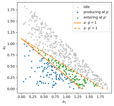
Fig. 42.1 Cells that enter when \(p_1\) falls#
producing at p  : 102 cells, X1/X2 = 1.81
entering at p'  :  93 cells, X1/X2 = 2.82
producing at p' : 195 cells, X1/X2 = 2.31
The price line pivots on its intercept with the \(a_2\) axis, so the cells that enter lie in a wedge that opens toward the \(a_1\) axis.
On average they use more of input 1, relative to input 2, than the cells already producing.
The industry’s ratio \(X_1/X_2\) therefore rises when input 1 becomes cheaper, although no cell changes its own input mix.
42.5.4. Checking efficiency#
Next we check Theorem 42.1 on a sample of cells.
At prices \(p = (1, 1)\), we let each cell maximize profit, add up the cells’ outputs and inputs, and solve the linear program at those total inputs.
rng = np.random.default_rng(1234)
a, c = draw_cells(3000, A, α, ā, rng)

p = np.array([1.0, 1.0])
active = a @ p < 1
X0_cells = c[active].sum()
X_cells = (a[active] * c[active, None]).sum(axis=0)
F_value, duals = F_lp(X_cells, a, c)
print(f"output when each cell maximizes profit: {X0_cells:.6f}")
print(f"largest attainable output F_N(X):      {F_value:.6f}")
print(f"dual prices:                           "
      f"({duals[0]:.4f}, {duals[1]:.4f})")
output when each cell maximizes profit: 0.079878
largest attainable output F_N(X):      0.079878
dual prices:                           (1.0026, 0.9923)
The two outputs agree, as Theorem 42.1 says they must.
The dual prices are close to, but not exactly, the prices \(p = (1, 1)\) that the cells faced.
With finitely many cells, a small set of prices supports the same choices by all cells, and the solver reports one of them.
\(p = (1, 1)\) is also in that set: at those prices the dual objective \(p \cdot X + \Pi_N(p)\) in (42.8) equals the output of the cells that produce.
42.5.5. Comparing with Cobb–Douglas#
Now we compare \(F_N\) with Houthakker’s Cobb–Douglas function, at the totals \(X(p)\) from (42.4).
print(f"{'p':12} {'F_N(X(p))':>10} {'Cobb-Douglas':>13}   dual prices")
for p in [(1.0, 1.0), (0.7, 1.6), (1.3, 0.8)]:
    X0, X1, X2 = pareto_totals(p, A, α)
    F_value, duals = F_lp([X1, X2], a, c)
    print(f"{str(p):12} {F_value:10.4f} {X0:13.4f}   "
          f"({duals[0]:.3f}, {duals[1]:.3f})")
p             F_N(X(p))  Cobb-Douglas   dual prices
(1.0, 1.0)       0.0762        0.0762   (1.036, 0.985)
(0.7, 1.6)       0.0767        0.0768   (0.700, 1.657)
(1.3, 0.8)       0.0624        0.0630   (1.335, 0.752)
With 3,000 cells, of which a few hundred produce, \(F_N\) is within a percent of the Cobb–Douglas function at these three price vectors, and the dual prices are within about 6 percent of the prices that generate \(X(p)\).
Part of that is luck.
Output depends on the few hundred cells that produce, and across random samples of 3,000 cells the gap between \(F_N\) and the Cobb–Douglas function has a standard deviation of about 2 percent.
The figure compares isoquants.
We restrict the inputs to a region where the Cobb–Douglas prices satisfy \(p_i \geq 1/\bar a_i\), so that the truncated distribution has the same aggregate production function (42.6) as the full one.
X0_ref, X1_ref, X2_ref = pareto_totals((1.0, 1.0), A, α)
levels = X0_ref * np.array([0.8, 1.0, 1.2])

fig, axes = plt.subplots(1, 2, figsize=(10, 4.5), sharey=True)
for ax, N, n_grid in zip(axes, (100, 3000), (80, 30)):
    rng = np.random.default_rng(0)
    a, c = draw_cells(N, A, α, ā, rng)
    x1 = np.linspace(0.5, 1.6, n_grid) * X1_ref
    x2 = np.linspace(0.5, 1.6, n_grid) * X2_ref
    F_grid = np.array([[F_lp([u, v], a, c)[0] for u in x1] for v in x2])
    G1, G2 = np.meshgrid(x1, x2)
    ax.contour(G1, G2, cobb_douglas(G1, G2, A, α), levels=levels,
               colors="0.4", linestyles="--", linewidths=1)
    ax.contour(G1, G2, F_grid, levels=levels, colors="C0", linewidths=2)
    ax.plot([], [], color="C0", lw=2, label=r"$F_N$")
    ax.plot([], [], color="0.4", lw=1, ls="--", label="Cobb–Douglas")
    ax.set_title(f"{N:,} cells")
    ax.set_xlabel(r"$X_1$")
    ax.legend(loc="upper right")
axes[0].set_ylabel(r"$X_2$")
plt.show()
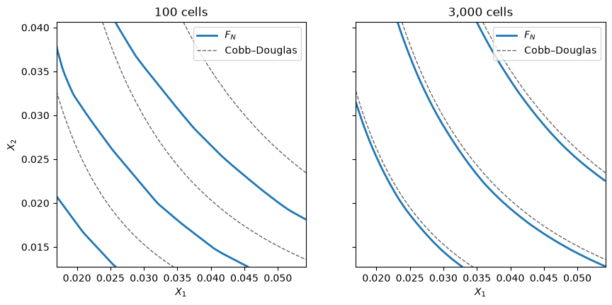
Fig. 42.2 Isoquants of \(F_N\) and Cobb–Douglas#
With 100 cells, only about ten run at any point of the grid, so the isoquants are visibly polygonal.
In this sample they also lie well inside the Cobb–Douglas isoquants, which means more output from the same inputs.
That is luck: across samples of 100 cells, the gap between \(F_N\) and the Cobb–Douglas function has a standard deviation of about 9 percent.
With 3,000 cells, they are smooth and close to the isoquants of (42.6).
The remaining gap, a percent or two of output, is sampling error, and its sign changes from sample to sample.
42.6. Levhari’s inverse problem#
Houthakker went from a distribution of cells to an aggregate production function.
Levhari [1968] went the other way: given an aggregate production function, which distribution of cells generates it?
If the answer exists for every reasonable production function, then Houthakker’s construction is not a special device for Cobb–Douglas but a way to read any aggregate production function as the sum of fixed-proportions cells.
Like Levhari, we simplify to one variable input, which we call labor, so that the inverse problem becomes one-dimensional.
42.6.1. One variable input#
Each cell needs \(t\) units of labor to produce one unit of output, and \(g(t) \, dt\) is the total capacity of the cells whose requirements lie between \(t\) and \(t + dt\).
Here \(t\) plays the role of the coefficient \(a\) and \(g\) the role of \(\varphi\): Houthakker’s one-input distribution is \(g(t) = A t^{\alpha - 1}\).
At a wage \(w\), measured in units of output, a cell produces if \(t < 1/w\).
Let \(x = 1/w\) be the requirement of the marginal cell.
The industry’s output and employment are
These are the \(X_0\) and \(X_1\) of (42.1) for one input whose price is \(w\).
As \(x\) varies, \((L, Q)\) traces out the aggregate production function \(Q = F(L)\).
Levhari observes that this relation is a Lorenz curve.
If we line the cells up from the lowest requirement to the highest, \(Q\) is the capacity of the first cells in line and \(L\) is the labor they use.
So \(L\) as a function of \(Q\) is an unnormalized Lorenz curve of labor requirements, weighted by capacity, as in Wealth Distribution Dynamics.
It is convex because requirements rise along the line, which makes \(F\) concave.
Differentiating (42.9) gives
The marginal product of labor is the productivity of the marginal cell, and it equals the wage, as Theorem 42.1 requires.
42.6.2. Inverting the aggregate production function#
This relation solves the inverse problem.
Given a concave, increasing \(F\), the marginal cell at employment \(L\) has requirement \(x = 1/F'(L)\), and the cells with requirements below \(x\) produce \(F(L)\):
Equivalently, the cell in position \(Q\) along the line needs \(1 / F'(F^{-1}(Q))\) units of labor.
Differentiating (42.10) with respect to \(L\) gives the density of capacity:
Capacity is dense where the production function is nearly linear.
If many cells share almost the same requirement, the marginal product barely falls as labor is added, so \(F''\) is small.
As a check, take Houthakker’s Cobb–Douglas case, \(F(L) = L^\gamma\).
Then \(F'(L) = \gamma L^{\gamma - 1} = 1/x\) gives \(L = (\gamma x)^{1/(1 - \gamma)}\), and (42.10) gives
This is the one-input version of (42.3) with \(\alpha = \gamma / (1 - \gamma)\), which is equivalent to \(\gamma = \alpha / (1 + \alpha)\), as in (42.5).
42.6.3. The CES case#
Levhari applies the inversion to the CES production function
Levhari writes \(\alpha\) for our \(\gamma\), \(A\) for our \(L\), \(p\) for our wage \(w\), and \(\phi\) and \(\psi\) for our \(G\) and \(H\).
We write \(\gamma\) for the weight on labor because, when \(\gamma + \beta = 1\), it becomes the Cobb–Douglas exponent as \(\rho \to 0\).
The constant \(\beta\) represents the fixed input, set to one, so \(F(L) = \tilde F(L, 1)\) with \(\tilde F(L, K) = (\gamma L^\rho + \beta K^\rho)^{1/\rho}\).
The elasticity of substitution between labor and the fixed input is \(\sigma = 1/(1 - \rho)\), which is less than one.
If \(\rho\) were positive, \(F(0) = \beta^{1/\rho}\) would be positive: the industry could produce without labor, which Houthakker’s assumptions rule out.
Two properties of (42.12) shape the distribution.
The average product \(F(L)/L = (\gamma + \beta L^{-\rho})^{1/\rho}\) falls from \(\gamma^{1/\rho}\) as \(L\) rises from zero, so no cell needs less than \(x_{\min} = \gamma^{-1/\rho}\) units of labor per unit of output.
As \(L \to \infty\), \(F(L) \to \beta^{1/\rho}\), so total capacity is finite.
To solve (42.10), write \(v = (x_{\min}/x)^{1 - \sigma}\) and use \(\rho = 1 - 1/\sigma\).
At the marginal cell, \(F'(L) = \gamma (F(L)/L)^{1 - \rho} = 1/x\), so the average product is \(F(L)/L = (\gamma x)^{-\sigma}\).
Then \(\gamma (L/F(L))^\rho = \gamma (\gamma x)^{\sigma - 1} = v\), because \(x_{\min}^{1 - \sigma} = \gamma^\sigma\).
Dividing \(F(L)^\rho = \gamma L^\rho + \beta\) by \(F(L)^\rho\) gives \(1 = v + \beta F(L)^{-\rho}\), and (42.10) then gives
This is Levhari’s equation (7), rewritten.
Dividing by total capacity \(\beta^{1/\rho}\) gives a probability distribution of requirements.
Differentiating gives the density of capacity:
The exponent \((2\sigma - 1)/(1 - \sigma)\) determines what happens at the lowest requirement \(x_{\min}\), where the bracket vanishes.
If \(1/2 < \sigma < 1\), the exponent is positive and \(g(x) \to 0\) as \(x \downarrow x_{\min}\).
If \(\sigma = 1/2\), the exponent is zero and \(g(x_{\min}) = \beta^{1/\rho} \sigma / x_{\min} = 1/(2 \gamma \beta)\); the normalized density plotted below starts at \(\sigma / x_{\min} = 1/(2\gamma)\).
If \(\sigma < 1/2\), the exponent is negative and \(g(x) \to \infty\) as \(x \downarrow x_{\min}\).
These cases make economic sense.
As \(\sigma \to 0\), the CES function approaches a fixed-proportions function, and the cells approach a single type with requirement \(x_{\min}\), so capacity piles up there.
As \(\sigma\) rises toward one, requirements are more dispersed, and few cells sit near the minimum.
Note
Levhari’s text and his Figure 1 get the first and third cases the wrong way around: he says that \(g(x) \to \infty\) at \(x_{\min}\) when \(-1 < \rho < 0\) and \(g(x) \to 0\) when \(\rho < -1\).
His own formula (8) gives the right answer, because its bracket vanishes at \(x_{\min}\) and carries the exponent \(-(1 + \rho)/\rho = (2\sigma - 1)/(1 - \sigma)\), which is positive when \(-1 < \rho < 0\).
His gloss “(i.e., \((1 + \rho)/\rho < 0\))” suggests that the minus sign in front of the exponent was dropped when the cases were read off.
Formula (8) also puts \(\beta^{1/\rho}\) in the denominator: the derivative of his (7) has \(\beta^{1/\rho}\) in the numerator, as in (42.14), and the normalized density has no \(\beta\), so (8) is right only when \(\beta = 1\).
His Figure 1 gives the border-case density as \(\gamma^{1/2} x^{-3/2} / (2 \beta)\), in our notation, which agrees with (42.14).
The code below implements the CES function, the closed forms (42.13) and (42.14), and the general inversion (42.10), which solves \(F'(L) = 1/x\) numerically.
The closed forms are coded through \(v\), computed as \((\gamma x^\rho)^{1/(1 - \rho)}\), which equals \((x_{\min}/x)^{1 - \sigma}\).
This avoids the very large number \(\beta^{1/\rho}\) and the very small number \(x_{\min}\) when \(\rho\) is near zero.
def ces(L, γ, β, ρ):
    return (γ * L**ρ + β)**(1 / ρ)


def ces_marginal_product(L, γ, β, ρ):
    return γ * (ces(L, γ, β, ρ) / L)**(1 - ρ)


def ces_capacity(x, γ, β, ρ):
    """G(x) from (ha_ces_dist), written as (β / (1 - v))**(1/ρ)."""
    v = (γ * x**ρ)**(1 / (1 - ρ))       # equals (x_min / x)**(1 - σ)
    return (β / (1 - v))**(1 / ρ)


def ces_density(x, γ, β, ρ):
    """g(x) from (ha_ces_density), written as (σ/x) (v/(1 - v)) G(x)."""
    σ = 1 / (1 - ρ)
    v = (γ * x**ρ)**(1 / (1 - ρ))
    return σ / x * v / (1 - v) * ces_capacity(x, γ, β, ρ)


def capacity_by_inversion(x, F, F_prime, L_bounds=(1e-12, 1e12)):
    """G(x) from (ha_inversion): find L with F'(L) = 1/x, return F(L)."""
    L = brentq(lambda L: F_prime(L) - 1 / x, *L_bounds,
               xtol=1e-14, rtol=1e-12)
    return F(L)


def levhari_7(x, γ, β, ρ):
    """Levhari's equation (7), in our notation."""
    z = (γ * x)**(ρ / (ρ - 1))
    return (β * z / (z - γ))**(1 / ρ)
We check that the three expressions for \(G\) agree and that (42.14) is the derivative of (42.13).
We use \(\gamma = 0.6\) and \(\beta = 0.4\) throughout; \(\gamma + \beta = 1\) will matter below.
γ, β = 0.6, 0.4

print(f"{'ρ':<6}{'closed - inversion':>20}{'closed - Levhari (7)':>22}"
      f"{'g/(dG/dx) - 1':>15}")
for ρ in (-0.5, -1.0, -2.0):
    x_min = γ**(-1 / ρ)
    xs = x_min * np.array([1.01, 1.5, 3.0, 10.0])
    G_closed = ces_capacity(xs, γ, β, ρ)
    G_inv = [capacity_by_inversion(
                 x, lambda L: ces(L, γ, β, ρ),
                 lambda L: ces_marginal_product(L, γ, β, ρ)) for x in xs]
    h = 1e-6
    g_numeric = (ces_capacity(xs * (1 + h), γ, β, ρ)
                 - ces_capacity(xs * (1 - h), γ, β, ρ)) / (2 * h * xs)
    e1 = np.max(np.abs(G_closed - G_inv))
    e2 = np.max(np.abs(G_closed - levhari_7(xs, γ, β, ρ)))
    e3 = np.max(np.abs(ces_density(xs, γ, β, ρ) / g_numeric - 1))
    print(f"{ρ:<6}{e1:>20.1e}{e2:>22.1e}{e3:>15.1e}")
ρ       closed - inversion  closed - Levhari (7)  g/(dG/dx) - 1
-0.5               8.0e-15               4.4e-16        1.6e-10
-1.0               3.9e-16               2.2e-16        1.5e-10
-2.0               9.9e-14               7.5e-16        1.4e-09
Here are the densities of the normalized distributions \(G/\beta^{1/\rho}\) for three elasticities of substitution.
Compare them with Levhari’s Figure 1, which has the first and third shapes reversed.
fig, axes = plt.subplots(1, 3, figsize=(10, 3.4))
for ax, ρ in zip(axes, (-0.5, -1.0, -2.0)):
    σ = 1 / (1 - ρ)
    x_min = γ**(-1 / ρ)
    xs = x_min * (1 + np.geomspace(1e-4, 4, 400))
    density = ces_density(xs, γ, β, ρ) / β**(1 / ρ)
    ax.plot(xs, density, lw=2)
    ax.axvline(x_min, color="0.5", lw=1, ls="--")
    ax.set_title(rf"$\rho = {ρ}$, $\sigma = {σ:.2f}$")
    ax.set_xlabel("labor requirement $x$")
    ax.set_xlim(0, 5 * x_min)
    ax.set_ylim(0, 1.6 * density[xs > 1.05 * x_min].max())
    if σ < 0.5:
        ax.annotate(r"$\to \infty$", xy=(x_min, ax.get_ylim()[1]),
                    xytext=(6, -14), textcoords="offset points")
axes[0].set_ylabel("density")
plt.tight_layout()
plt.show()
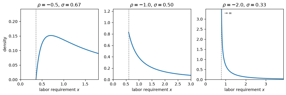
Fig. 42.3 Densities that generate CES functions#
The dashed lines mark \(x_{\min}\), and each panel has its own vertical scale.
With \(\sigma = 2/3\) the density starts at zero; with \(\sigma = 1/2\) it starts at a finite value; with \(\sigma = 1/3\) it is unbounded at \(x_{\min}\), and the plot cuts it off.
For an independent check, we draw cells from (42.13) and aggregate them as in (42.9).
Inverting (42.13) gives the requirement of a cell whose quantile in the normalized distribution is \(u \in (0, 1)\):
def draw_requirements(N, γ, ρ, rng):
    """Draw N labor requirements from the normalized distribution."""
    σ = 1 / (1 - ρ)
    u = rng.random(N)
    return γ**(-1 / ρ) * (1 - u**((1 - σ) / σ))**(-1 / (1 - σ))
We sort the cells from the lowest requirement to the highest and give each an equal share of total capacity \(\beta^{1/\rho}\).
The cumulative sums trace out the aggregate production function.
rng = np.random.default_rng(2)
N = 20_000
L_grid = np.linspace(1e-3, 6, 200)

fig, ax = plt.subplots()
for ρ, color in zip((-0.5, -2.0), ("C0", "C1")):
    t = np.sort(draw_requirements(N, γ, ρ, rng))
    capacity = β**(1 / ρ) / N
    Q = capacity * np.arange(1, N + 1)
    L = capacity * np.cumsum(t)
    keep = L <= L_grid[-1]
    ax.plot(L[keep], Q[keep], color=color, lw=4, alpha=0.4,
            label=rf"{N:,} cells, $\rho = {ρ}$")
    ax.plot(L_grid, ces(L_grid, γ, β, ρ), color=color, lw=1, ls="--",
            label=rf"CES, $\rho = {ρ}$")
ax.set_xlabel("labor $L$")
ax.set_ylabel("output $Q$")
ax.legend()
plt.show()
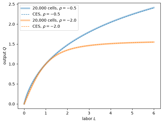
Fig. 42.4 Aggregating cells drawn from Levhari’s distributions#
The aggregated cells reproduce the CES functions.
42.6.4. The Cobb–Douglas limit#
As \(\rho \to 0\), the CES function (42.12) with \(\gamma + \beta = 1\) approaches \(L^\gamma\).
Levhari uses l’Hôpital’s rule to show that \(G\) then approaches the power law \((\gamma x)^{\gamma/(1 - \gamma)}\), so the CES distributions approach Houthakker’s.
(He does not state the condition \(\gamma + \beta = 1\), but the limit needs it: otherwise \((\gamma L^\rho + \beta)^{1/\rho}\) goes to zero or to infinity as \(\rho \to 0\).)
Along the way \(x_{\min} = \gamma^{-1/\rho}\) falls to zero.
xs = np.array([0.5, 1.0, 2.0, 4.0])
print(f"{'power law':12}", np.round((γ * xs)**(γ / (1 - γ)), 5))
for ρ in (-0.1, -0.01, -0.001, -1e-5):
    print(f"ρ = {ρ:<8}", np.round(ces_capacity(xs, γ, β, ρ), 5))
power law    [0.16432 0.46476 1.31453 3.71806]
ρ = -0.1     [0.14874 0.47726 1.27581 2.96343]
ρ = -0.01    [0.16281 0.46604 1.31018 3.61928]
ρ = -0.001   [0.16417 0.46489 1.31409 3.70787]
ρ = -1e-05   [0.16432 0.46476 1.31453 3.71796]
Both papers’ distributions have very fat upper tails.
In Houthakker’s, total capacity is infinite; in Levhari’s, total capacity is finite but the mean requirement is infinite, as Exercise 42.3 asks you to show.
42.7. Later work#
Levhari [1968] opens by noting that Houthakker’s paper had been neglected, as Solow [1967] had observed in his survey of production theory.
Its central idea has since been taken up in several directions.
Johansen [1972] made Houthakker’s construction the basis of a theory of short-run industry production functions, derived from the distribution of capacity over the input coefficients of fixed-proportions production units.
He combined it with a putty-clay vintage model in which investment in new units shifts that distribution over time.
Hildenbrand [1981] studied the construction with many inputs and outputs and showed that the industry’s short-run production set is a zonoid.
With finitely many cells, that set is a sum of line segments, one from the origin to each cell’s input–output vector at full capacity, and with a continuum of cells it is a limit of such sums.
Jones [2005] treated ideas as techniques, Leontief in his analytical model, whose labor and capital coefficients are drawn from independent Pareto distributions.
His global production function is the upper envelope of the techniques discovered, not a sum over capacity-constrained cells, so it has constant returns.
He showed that its expected value is Cobb–Douglas and that long-run technical change is labor-augmenting, and he contrasts his construction with Houthakker’s.
Lagos [2006] combined Houthakker’s aggregation with a frictional labor market in which jobs are created and destroyed, so that labor-market policies affect measured total factor productivity by changing which cells operate.
42.8. Concluding remarks#
Houthakker’s construction separates two things that an aggregate production function runs together: the technology of each cell and the distribution of technologies across cells.
No cell can substitute one input for another, yet the industry can, because a change in relative prices changes which cells operate.
The form of the aggregate function is a property of the distribution: a Pareto distribution gives Cobb–Douglas, and with one variable input Levhari’s inversion finds a distribution of cells behind any smooth, increasing, strictly concave production function with \(F(0) = 0\).
Because the aggregate function depends on how the fixed inputs are spread across cells, it describes the short run and moves when entry, exit or investment changes that spread.
That is why Houthakker warned against adding the fixed inputs as one more argument of the function, and why he closed his note by asking for data on the distribution of input–output ratios across firms and machines, such as cotton spindles.
42.9. Exercises#
Exercise 42.1
We saw that Houthakker’s distribution (42.3) scales as a power separately in \(a_1\) and in \(a_2\).
This exercise shows that scaling jointly in \((a_1, a_2)\) is not enough for a Cobb–Douglas aggregate production function.
Consider
which is homogeneous of degree \(\kappa - 2\).
Let \(s_i = p_i X_i / X_0\) be the share of input \(i\) (in Houthakker’s case, \(s_i = \gamma_i\)).
Show that \(X_0(\lambda p) = \lambda^{-\kappa} X_0(p)\) and \(X_i(\lambda p) = \lambda^{-\kappa - 1} X_i(p)\), and conclude that \(F\) is homogeneous of degree \(\kappa/(1 + \kappa)\) and that \(s_1 + s_2 = \kappa/(1 + \kappa)\).
Change variables to \(r = a_1 + a_2\) and \(u = a_1 / r\) to reduce (42.1) to one-dimensional integrals over \(u \in [0, 1]\).
Compute the share \(s_1\) as \(p_1/p_2\) ranges from \(0.1\) to \(10\) for \(\kappa = 1\), \(2\) and \(4\). For which \(\kappa\) is \(F\) Cobb–Douglas? For a production function that is homogeneous, the elasticity of substitution between the two inputs is \(\sigma_{12} = 1 - d \log(s_1/s_2) / d \log(p_1/p_2)\). Compute it, and explain why it is below one for \(\kappa = 1\) and above one for \(\kappa = 4\). Hint: along each line \(a_1 + a_2 = r\), compare how \(\varphi\) and Houthakker’s distribution \(a_1^{\kappa/2 - 1} a_2^{\kappa/2 - 1}\), which is homogeneous of the same degree, spread capacity over the input mix \(u = a_1/r\).
Solution
Here is one solution.
For part 1, substitute \(a = \lambda^{-1} \tilde a\) in (42.1) at prices \(\lambda p\).
The region \(a \cdot \lambda p < 1\) becomes \(\tilde a \cdot p < 1\), \(da = \lambda^{-2} d\tilde a\), and \(\varphi(\lambda^{-1} \tilde a) = \lambda^{2 - \kappa} \varphi(\tilde a)\), so \(X_0(\lambda p) = \lambda^{-\kappa} X_0(p)\).
The extra factor \(a_i = \lambda^{-1} \tilde a_i\) gives \(X_i(\lambda p) = \lambda^{-\kappa - 1} X_i(p)\).
Scaling prices by \(\lambda\) therefore scales inputs by \(\lambda^{-\kappa - 1}\) and output by \(\lambda^{-\kappa} = (\lambda^{-\kappa - 1})^{\kappa/(1 + \kappa)}\), so \(F\) is homogeneous of degree \(\kappa/(1 + \kappa)\).
Because marginal products equal prices, Euler’s theorem gives \(p_1 X_1 + p_2 X_2 = \frac{\kappa}{1 + \kappa} X_0\).
For part 2, \(a_1 = r u\) and \(a_2 = r(1 - u)\) have Jacobian \(r\), and the price triangle becomes \(r < R(u) \equiv 1/(u p_1 + (1 - u) p_2)\).
Integrating over \(r\) gives
def homogeneous_totals(p, κ):
    p1, p2 = p
    R = lambda u: 1 / (u * p1 + (1 - u) * p2)
    X0 = integrate.quad(lambda u: R(u)**κ, 0, 1)[0] / κ
    X1 = integrate.quad(lambda u: u * R(u)**(κ + 1), 0, 1)[0] / (κ + 1)
    X2 = integrate.quad(lambda u: (1 - u) * R(u)**(κ + 1), 0, 1)[0] / (κ + 1)
    return X0, X1, X2


κ = 4.0
p = (0.5, 1.0)
print("one-dimensional:", np.round(homogeneous_totals(p, κ), 10))
print("two-dimensional:", np.round(totals_by_quadrature(
    p, lambda a1, a2: (a1 + a2)**(κ - 2)), 10))
one-dimensional: [1.16666667 1.13333333 0.36666667]
two-dimensional: [1.16666667 1.13333333 0.36666667]
For part 3, we compute the shares and the elasticity of substitution on a grid of price ratios.
We also compute \(\sigma_{12}\) at equal prices with a small centered difference.
def log_share_ratio(r, κ):
    """log(s1/s2) at prices (r, 1)."""
    X0, X1, X2 = homogeneous_totals((r, 1.0), κ)
    return np.log(r * X1 / X2)


ratios = np.geomspace(0.1, 10, 41)
h = 1e-4

fig, axes = plt.subplots(1, 2, figsize=(10, 4))
for κ in (1.0, 2.0, 4.0):
    shares = []
    for r in ratios:
        X0, X1, X2 = homogeneous_totals((r, 1.0), κ)
        shares.append((r * X1 / X0, X2 / X0))
    s1, s2 = np.array(shares).T
    σ12 = 1 - np.gradient(np.log(s1 / s2), np.log(ratios), edge_order=2)
    σ12_equal = 1 - (log_share_ratio(np.exp(h), κ)
                     - log_share_ratio(np.exp(-h), κ)) / (2 * h)
    print(f"κ = {κ}: s1 + s2 in [{(s1 + s2).min():.4f}, "
          f"{(s1 + s2).max():.4f}], κ/(1+κ) = {κ / (1 + κ):.4f}; "
          f"σ12 at p1 = p2: {σ12_equal:.4f}")
    axes[0].plot(ratios, s1, lw=2, label=rf"$\kappa = {κ:g}$")
    axes[1].plot(ratios, σ12, lw=2, label=rf"$\kappa = {κ:g}$")
axes[0].set_ylabel("share of input 1")
axes[1].set_ylabel("elasticity of substitution")
for ax in axes:
    ax.set_xscale("log")
    ax.set_xlabel(r"$p_1 / p_2$")
    ax.legend()
plt.tight_layout()
plt.show()
κ = 1.0: s1 + s2 in [0.5000, 0.5000], κ/(1+κ) = 0.5000; σ12 at p1 = p2: 0.6667
κ = 2.0: s1 + s2 in [0.6667, 0.6667], κ/(1+κ) = 0.6667; σ12 at p1 = p2: 1.0000
κ = 4.0: s1 + s2 in [0.8000, 0.8000], κ/(1+κ) = 0.8000; σ12 at p1 = p2: 1.6667
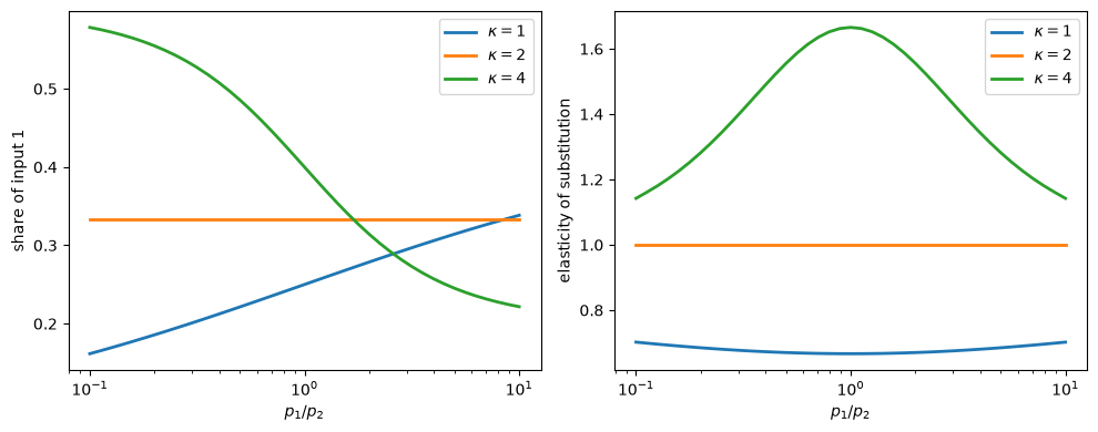
Fig. 42.5 Shares and elasticities under homogeneous \(\varphi\)#
The shares add up to \(\kappa/(1 + \kappa)\) for every price ratio, as part 1 predicts.
Only for \(\kappa = 2\) is the share of input 1 constant, at \(1/3\), so only then is \(F\) Cobb–Douglas.
That is no coincidence: with \(\kappa = 2\), \(\varphi\) is constant, which is Houthakker’s distribution (42.3) with \(\alpha_1 = \alpha_2 = 1\).
For \(\kappa = 1\) the share of input 1 rises with its relative price, so \(\sigma_{12} < 1\).
For \(\kappa = 4\) the share falls with its relative price, so \(\sigma_{12} > 1\).
At equal prices the elasticities are \(2/3\) and \(5/3\).
To see why, recall that aggregate substitution happens because a change in relative prices switches cells on and off.
Switching cells whose input mix is extreme, near the axes, changes the industry’s input mix the most.
Along each line \(a_1 + a_2 = r\), \(\varphi\) spreads capacity evenly over the mix \(u = a_1/r\), while Houthakker’s distribution \(a_1^{\kappa/2 - 1} a_2^{\kappa/2 - 1}\) spreads it in proportion to \(u^{\kappa/2 - 1} (1 - u)^{\kappa/2 - 1}\).
When \(\kappa < 2\), that weight is largest near \(u = 0\) and \(u = 1\), so \(\varphi\) has relatively fewer cells with extreme mixes, and substitution is weaker than Cobb–Douglas.
When \(\kappa > 2\), that weight vanishes near \(u = 0\) and \(u = 1\), so \(\varphi\) has relatively more cells with extreme mixes, and substitution is stronger.
This can be made exact.
Suppose that \(\varphi(a) = r^{\kappa - 2} w(u)\) for a weight \(w\) that is symmetric about \(u = 1/2\), and set \(p_1 = e^\varepsilon\) and \(p_2 = 1\).
Then \(R(u)^{\kappa + 1} \approx 1 - (1 + \kappa) u \varepsilon\), and with \(\mathbb{E}\) denoting averages over \(u\) with weights proportional to \(w\), so that \(\mathbb{E} u = 1/2\),
Since \(s_1/s_2 = e^\varepsilon X_1/X_2\), at equal prices
For our \(\varphi\), \(w\) is uniform and \(\operatorname{Var}(u) = 1/12\), which gives \(\sigma_{12} = (1 + \kappa)/3\), matching the computed \(2/3\) and \(5/3\).
For Houthakker’s distribution, \(w\) is a Beta\((\kappa/2, \kappa/2)\) density with variance \(1/(4(1 + \kappa))\), which gives \(\sigma_{12} = 1\).
At equal prices, the elasticity of substitution is proportional to the dispersion of input mixes across cells.
Exercise 42.2
Return to one variable input.
Write the aggregate production function as \(F(L) = \tilde F(L, 1)\), where \(\tilde F(L, K) = K F(L/K)\) is homogeneous of degree one, and let
be labor’s share of output and the elasticity of substitution between labor and the fixed input.
Use (42.10) to show that the elasticity \(d \log G / d \log x = x g(x)/G(x)\) of the capacity distribution with respect to the requirement of the marginal cell is
\[ \frac{x \, g(x)}{G(x)} = \sigma(L) \, \frac{s(L)}{1 - s(L)}, \qquad \text{where } F'(L) = 1/x . \]Use this identity to show that a Cobb–Douglas function \(F(L) = C L^\gamma\) requires \(G(x) \propto x^{\gamma/(1 - \gamma)}\). Then show directly from (42.9) that every power law \(G(x) = k x^\alpha\) generates a Cobb–Douglas function. So, with one variable input, Houthakker’s distribution is the only one that yields a Cobb–Douglas function.
Check the identity numerically for the CES function (42.12).
Solution
Here is one solution.
For part 1, write \(x(L) = 1/F'(L)\), so that (42.10) reads \(G(x(L)) = F(L)\).
Take logarithms and differentiate with respect to \(L\):
Hence
The definition of \(\sigma\) gives \(-F F'' = F'(F - L F') / (\sigma L)\), and substituting,
For part 2, a Cobb–Douglas function has \(\sigma = 1\) and \(s = \gamma\) at every \(L\), and its marginal product \(F'(L) = C \gamma L^{\gamma - 1}\) takes every positive value as \(L\) ranges over \((0, \infty)\).
The identity then says that \(x g(x)/G(x) = \gamma/(1 - \gamma)\) for every \(x > 0\), so \(\log G\) is linear in \(\log x\) with slope \(\gamma/(1 - \gamma)\).
Conversely, if \(G(x) = k x^\alpha\), then \(g(x) = k \alpha x^{\alpha - 1}\), and (42.9) gives \(Q = k x^\alpha\) and \(L = k \alpha x^{\alpha + 1}/(\alpha + 1)\).
Eliminating \(x\),
which is Cobb–Douglas with \(\gamma = \alpha/(1 + \alpha)\).
For part 3, the CES function has \(\sigma = 1/(1 - \rho)\) at every \(L\), while labor’s share varies.
for ρ in (-0.5, -1.0, -2.0):
    σ = 1 / (1 - ρ)
    for L in (0.1, 1.0, 10.0):
        F_L = ces(L, γ, β, ρ)
        mp = ces_marginal_product(L, γ, β, ρ)
        x, s = 1 / mp, L * mp / F_L
        lhs = x * ces_density(x, γ, β, ρ) / ces_capacity(x, γ, β, ρ)
        print(f"ρ = {ρ:5}, L = {L:5}: x g/G = {lhs:9.6f}, "
              f"σ s/(1 - s) = {σ * s / (1 - s):9.6f}")
ρ =  -0.5, L =   0.1: x g/G =  3.162278, σ s/(1 - s) =  3.162278
ρ =  -0.5, L =   1.0: x g/G =  1.000000, σ s/(1 - s) =  1.000000
ρ =  -0.5, L =  10.0: x g/G =  0.316228, σ s/(1 - s) =  0.316228
ρ =  -1.0, L =   0.1: x g/G =  7.500000, σ s/(1 - s) =  7.500000
ρ =  -1.0, L =   1.0: x g/G =  0.750000, σ s/(1 - s) =  0.750000
ρ =  -1.0, L =  10.0: x g/G =  0.075000, σ s/(1 - s) =  0.075000
ρ =  -2.0, L =   0.1: x g/G = 50.000000, σ s/(1 - s) = 50.000000
ρ =  -2.0, L =   1.0: x g/G =  0.500000, σ s/(1 - s) =  0.500000
ρ =  -2.0, L =  10.0: x g/G =  0.005000, σ s/(1 - s) =  0.005000
The two sides agree.
Dividing (42.14) by (42.13) gives \(x g(x)/G(x) = \sigma v/(1 - v)\) with \(v = (x_{\min}/x)^{1 - \sigma}\), so the identity says that labor’s share is \(s = (x_{\min}/x)^{1 - \sigma}\) when the marginal cell needs \(x\) units of labor.
As \(x \downarrow x_{\min}\), labor’s share approaches one, and the elasticity of \(G\) grows without bound.
Exercise 42.3
Levhari notes that the distribution (42.13) has no finite mean.
Show that the normalized distribution \(P(x) = G(x)/\beta^{1/\rho}\) satisfies
\[ 1 - P(x) \approx \frac{\sigma}{1 - \sigma} \left( \frac{x_{\min}}{x} \right)^{1 - \sigma} \qquad \text{as } x \to \infty, \]so that its upper tail is a Pareto tail with index \(1 - \sigma < 1\), in the sense of Heavy-Tailed Distributions, and its mean is infinite.
Give an economic reason why the mean requirement must be infinite for any aggregate production function whose marginal product is positive at every \(L\) and whose total capacity is finite.
Draw \(100{,}000\) requirements with
draw_requirementsfor \(\rho = -0.5\), \(-1\) and \(-2\). Plot the empirical survival function \(1 - P\) on log-log axes, together with the approximation in part 1.
Solution
Here is one solution.
For part 1, let \(v = (x_{\min}/x)^{1 - \sigma}\), which goes to zero as \(x \to \infty\).
Then \(P(x) = (1 - v)^{\sigma/(1 - \sigma)} = 1 - \frac{\sigma}{1 - \sigma} v + O(v^2)\), which gives the approximation.
A distribution whose survival function falls like \(x^{-\zeta}\) has a finite mean only if \(\zeta > 1\).
Here \(\zeta = 1 - \sigma < 1\), so the mean is infinite.
For part 2, the industry’s employment is \(L = H(x)\), the labor used by all cells with requirements at most \(x\).
If the marginal product \(F'(L) = 1/x\) is positive at every \(L\), then every level of employment, however large, is reached at some finite \(x\).
So \(H(x) \to \infty\) as \(x \to \infty\): if every cell in the industry were operating, it would employ an infinite amount of labor.
With finite total capacity, that means an infinite mean requirement.
Levhari puts it this way: as the wage falls to zero, employment rises without bound because the marginal product of labor is always positive.
For part 3, we compare the empirical survival function with the approximation from part 1, shown as dashed lines.
rng = np.random.default_rng(3)
N = 100_000

fig, ax = plt.subplots()
for ρ, color in zip((-0.5, -1.0, -2.0), ("C0", "C1", "C2")):
    σ = 1 / (1 - ρ)
    x_min = γ**(-1 / ρ)
    t = np.sort(draw_requirements(N, γ, ρ, rng))
    survival = 1 - np.arange(1, N + 1) / N
    ax.loglog(t[:-1], survival[:-1], color=color, lw=2, alpha=0.6,
              label=rf"draws, $\sigma = {σ:.2f}$")
    x_grid = np.geomspace(10 * x_min, t[-2], 50)
    ax.loglog(x_grid, σ / (1 - σ) * (x_min / x_grid)**(1 - σ),
              color=color, lw=1, ls="--")
ax.set_xlabel("labor requirement $x$")
ax.set_ylabel(r"$1 - P(x)$")
ax.legend()
plt.show()
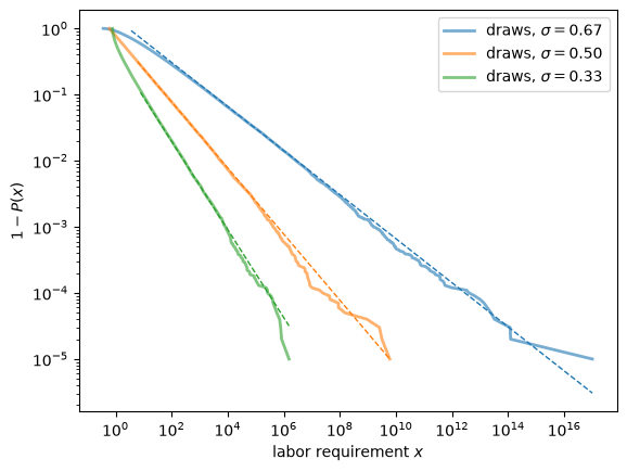
Fig. 42.6 Upper tails of Levhari’s distributions#
On log-log axes the survival functions become straight lines with slopes \(-(1 - \sigma)\), which are \(-1/3\), \(-1/2\) and \(-2/3\).
The smaller the elasticity of substitution, the thinner the tail, but even as \(\sigma \to 0\) the tail index stays below one.